This post is a guide to a Python implementation of the paper “Best Practices for Convolutional Neural Networks Applied to Visual Document Analysis” published by a Microsoft Research team. After a bit of theory about convolutional neural networks, we will code a 98.2%-accuracy convolutional network to classify images from the MNIST dataset. Then, we will create functions to preprocess the dataset to enhance our classifier accuracy, up to 99.6%. This guide is intended for readers relatively at ease with Python and the major concepts of neural networks (including backpropagation).
Introduction
About this post
The current part is intended to quickly introduce the context of this post. We will then overview the theory about convolutional networks needed to understand the finale code. In the third part of this post, we will create a 98.2%-accuracy classifier using tensorflow. Finally, we will implement a piece of code intended to preprocess the dataset to improve the network accuracy.
This is the first post of my new series "From Papers to Github": feedback will be greatly appreciated :-)
Prerequisites
- Python >= 2.7
- numpy >= 1.12.0 for data manipulation and image processing
- tensorflow >= 0.12.1 for training and implementing the convolutional network (doc)
- scipy >= 0.18.1 for dataset expansion
We will use tensorflow in this project because it is a well-documented and fast machine learning API. Plus, since it is developed by Google, there is a great chance it will be active for years. We could have used Theano which is also a great Python API for machine learning, but I feel like tensorflow is going to be vastly used in industry.
Quick overview of the paper
The reader is highly encouraged to read the associated paper to fully understand the context of this post.
Firstly, the paper depicts the architecture and the results of the convolutional network used by the research team. The network is made of 4-hidden layers and predicts the value of the digit written on an image with an accuracy of about 98%.
One of the methods to increase the accuracy of a neural network is to increase the size of the dataset used to train the network. We are going to create new images by applying affine and elastic distortions to every image of the starting dataset that are roughly representing the properties of the hand. The team achieved a 99.6% accuracy by combining this neural network with elastic distortions.
About the dataset
The famous MNIST dataset is used for the training and the validation of the classifier. This dataset consists of 28x28 labeled images of handwritten digits. It is split into two sets: a training set of 60000 images and a test set of 10000 images. Here is an example of 20 random images from the MNIST dataset :
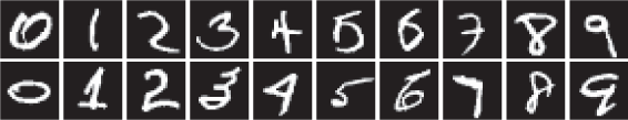
Figure 1 - Example of 2 random images for each class of digits from the MNIST dataset
A bit of theory
If you are confident with convolutional neural networks, feel free to skip the theory.
There are a lot of ways to introduce Convolutional Neural Networks. I am going to focus on the concept of layers rather than the one of neurons because I find it is suited to the analogy with filters when doing image processing (which is the case in this post). I recommend this excellent course if you want to fully understand convnets.
Convolutional Neural Networks
A Convolutional Neural Network (CNN), also shortened as convnet, is a type of Feedforward Neural Network. Hence, a CNN is a neural network that processes sequentially the input through layers that apply transformations to their inputs.
Convnets are usually constructed using four kinds of layers:
- FC: Fully Connected layer
- RELU: Rectified Linear Unit layer
- CONV: Convolutional layer
- POOL: Max-Pooling layer
A top-level model of a CNN is as follows :
In our case, the convnet used in the paper is implemented as follows:
Fully Connected layers
Fully Connected layers are usually used to extract high-level features from its inputs.
An FC is made of a set of neurons, a matrix of weights and a set of biases, where is a stricly positive integer chosen when modelizing the classifier. For each neuron of the layer, the forward pass producing the set of outputs given a set of inputs is computed with the dot addition between the dot product of the weights with the inputs and the biases:
For instance, here is a representation of a FC layer made of taking some input of size :
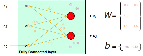
Figure 2 - Example of a FC layer
According to the previous formula, with an input , the computed outputs are:
During backpropagation, the weights and the biases are updated based on the expected output of the layer. For an in-depth explanation about backpropagation, I’d suggest you to look at some guides on the web (not treated here since it would vastly increase the size of this post).
ReLU layers
To generalize the behaviour of the network, a good custom is to apply non-linear functions to the transformations it applies to the input throughout each step of the forward propagation. These non-linear functions are also called activation functions. Since an activation function is applied to every output of a given layer, it can be seen as a layer itself of neurons where is the number of outputs from the previous layer i.e. the number of inputs of the current activation layer. The output of a RELU layer given an input and an activation function is:
Two of the most used activation functions are :

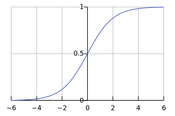
For instance, if we stack a RELU layer after the previous FC layer displayed in the example above, we end up with a neural network as follows:

Figure 3 - Example of a neural network made of one Fully Connected layer and one Rectified Linear Unit layer
Pursuing with the example, with a sigmoid function as activation function, we obtain the following outputs:
Convolutional layers
CONV layers are usually used to extract features from images. Indeed, they deal with inputs that have three dimensions: , and . For our purpose, the images are 28x28 greyscale pixels, so , and .
First of all, CONV layers are made of a set of weights, also called filters or kernels, of three dimensions, just like their inputs. The idea of a CONV layer is that we will compute a transformation of the input with every kernel so that we have a list of outputs, one for each kernel. More precisely, for each kernel, we will slide it throughout the and of the input and compute a dot multiplication followed by a bias addition.
The parameters of a CONV layer are :
- The number of filters .
- The size of every kernel. For example, with greyscale images and then the kernels are all of shape (1 because every pixel of a greyscale image has one dimension).
- The stride which represent the number of pixels a filter will skip when sliding through the input width dimensions and the input height dimension. More precisely, the filter will skip pixels for computing the next transformation, horizontally or vertically.
- The padding. We can add a border of 0 to the input so that the transformation of the filters will be applied properly to the border pixels.
We will look at some examples of CONV transformations instead of writing maths because it is quite a visual notion. In the following example, the input (the green matrix) is of shape . The filter (the orange matrix) is of shape and its values, displayed on the right bottom of every orange pixel (they are fixed), are . The padding is since we did not add any extra border of pixels of value 0. Finally, the stride is since the filter does not skip any pixel when sliding:
Figure 4 - Example of a CONV transformation (source)
For a more complete example, you can check this gif of a CONV layer with inputs, filters of size , padding equals to and stride equals to where the inputs have 3 channels (RGB).
A CONV layer will produce a set of outputs of shape with where is the output height/width, is the input height/width, is the filter height/width (i.e. filter size), is the padding and is the stride. (Don’t hesitate to try this formula with a pen and paper).
Max-Pool layers
We won’t use MAXPOOL layers for this project, but they are definitely a thing to improve some neural networks.
A MAXPOOL layer will slide a filter throughout the input, just like a CONV layer with just one filter. However, instead of performing dot multiplication followed by bias addition, a MAXPOOL layer will take the maximum from the local zone.
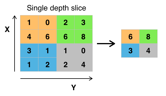
Figure 5 - Example of a MAXPOOL layer with 2x2 filter and stride of 2 (source)
Coding the classifier
Model implementation
For their research, the Microsoft team used a convnet with the following architecture:

Figure 6 - Model of the neuralnet depicted in the paper. RELU layers are not drawn (one after each layer except for input and output layers)
More precisely, here are the parameters for the CONV and FC layers :
| Shape of input | Number of filters | Shape of a filter | Stride | Padding | |
|---|---|---|---|---|---|
| CONV1 | 29x29x1 | 5 | 5x5x1 | 2 | 0 |
| CONV2 | 13x13x5 | 50 | 5x5x5 | 2 | 0 |
Regarding the size of the convolutional layers filters: CONV1 is stacked after the input witch has only 1 channel (greyscale images in the MNIST dataset); however CONV2 is stacked after CONV1 which, itself, has a depth of 5 (because it has 5 filters). Since a CONV layer compute local transformations at full depth, these filters have their third dimension equal to 5.
You may be wondering at this point why we switched from 28x28 pixel images to 29x29. This is due to the mixture between filters size, stride and padding: the size of the output is . In other words, this is due to natural CONV networks constraints (full explanation in the article). 29x29 images are the closest size in order to have an integer after our two CONV layers i.e. to have a valid convnet model.
| Shape of input | Number of neurons | |
|---|---|---|
| FC1 | 5x5x50 or 1250 | 100 |
| FC2 | 100 | 10 : digits from 0 to 9 |
Let’s start coding by importing the libraries we need for the network: tensorflow for convnet model and training, numpy for data manipulation and the dataset which can be retrieved from the tensorflow API:
import tensorflow as tf
import numpy as np
# tensorflow API to retrieve the MNIST dataset
# More info about MNIST here : http://yann.lecun.com/exdb/mnist/
from tensorflow.examples.tutorials.mnist import input_data
We are going to define the layers’ parameters before modeling them: they will be stocked in a dictionary for easy manipulation if we want to remodel the network. For both our CONV and FC layers, we need to define the weights and biases (for CONV layers, the weights are equivalent to the filters). In tensorflow, variables that are not constants (e.g. weights and biases since we want them to be modified with backpropagation) are defined using tf.Variable that takes a numpy array as input. Besides, we don’t want to initialize weights and biases with since in that case, the forward pass is worthless. Instead, we will use a normal initialization between (there are a lot of papers regarding the different ways to initialize weights and biases if you’re interested):
# Returns the parameters of the network used to build the model
def _net_params():
    weights = {
        # Example for conv1: 5 filters of size 5x5x1 -> shape (5, 5, 1, 5)
        # (last dim is the number of filters)
        'conv1': tf.Variable(tf.random_normal([5, 5, 1, 5])),
        'conv2': tf.Variable(tf.random_normal([5, 5, 5, 50])),
        'fc1': tf.Variable(tf.random_normal([5 * 5 * 50, 100])),
        'fc2': tf.Variable(tf.random_normal([100, 10])),
    }


    # Biases are added to the current layer's neurons
    # Consequently they are of same shape than the number of neurons of the layer
    biases = {
        'conv1': tf.Variable(tf.random_normal([5])),
        'conv2': tf.Variable(tf.random_normal([50])),
        'fc1': tf.Variable(tf.random_normal([100])),
        'fc2': tf.Variable(tf.random_normal([10])),
    }

    return weights, biases
As you can see, the CONV layers deal with variables of 4 dimensions while FC are defined with 2D variables. This is because the CONV layer will look at full-depth zones of the input. If you remember 2.1., the FC layers compute a global transformation of the input: the weights are dot multiplied to the full input then there is a bias add. In other words, FC layers look at all the previous neurons at once while CONV layers select zones. Consequently, we will need to reshape the output of CONV2 in order to feed it to FC1 (flatten a 4D vector into a 1D vector).
Now that we have the network parameters defined, we are going to create a function (also know as helper) that will automate the building of CONV, RELU and FC layers. More precisely, CONV layers will always be followed by a RELU layer in our network. FC1 will also be followed by an activation layer. However the output layer, i.e. FC2 will not be followed by a RELU layer (so we do not put it in the helper function).
# Helper to create a FC layer before activation
def _fc_layer(inputs, weights, biases):
    return tf.add(tf.matmul(inputs, weights), biases)


# Helper to create a CONV+RELU layer
def _conv_layer(inputs, weights, biases, stride=2, padding='VALID'):
    layer = tf.nn.conv2d(
        input=inputs,
        filter=weights,
        strides=[1, stride, stride, 1],
        padding=padding
    )
    # Adding biases to the filters fastforward transformations
    layer = tf.nn.bias_add(layer, biases)
    # Applying and returning RELU layer to CONV transformations + biases added
    return tf.nn.relu(layer)
padding=‘VALID’ means no-padding. In practice, we will see that the network will be fed a batch of images i.e. a list of images. Since we manipulate batch of images, inputs will be of 4 dimensions: batch dimension, image width dimension, image height dimension and pixel channels dimension. We don’t want to skip images (first dimension) nor channels (last dimension) so their associated dimension stride is 1. However, we want our “window” to split throughout by missing some pixels so we could want to put something other than for the height/width dimensions.
As you can see, we define the exact behaviour of FC layers by giving the mathematical operations to perform FC-computation. However, we use tf.nn.conv2d to perform the CONV layer transformation seen at 2.3.
We prepared everything we needed. Let’s build our model! (explanation below)
# Model of the convolutional network
# x: batch of images; shape (batch_size, 29, 29, 1)
def conv_net(x):
    # Retrieving layers' parameters
    weights, biases = _net_params()

    # Reshaping the inputs into 4 dimensions
    x = tf.reshape(x, shape=[-1, 28, 28, 1])
    # Adding an extra line and an extra column to every image of the batch
    x = tf.pad(x, paddings=[[0, 0], [0, 1], [0, 1], [0, 0]])

    # Conv layers
    conv1 = _conv_layer(x, weights['conv1'], biases['conv1'])
    conv2 = _conv_layer(conv1, weights['conv2'], biases['conv2'])

    # Flattening output of conv2 to be fed in fc1
    _fc1 = tf.reshape(conv2, [-1, weights['fc1'].get_shape().as_list()[0]])

    # Fully-connected layers
    fc1 = _fc_layer(_fc1, weights['fc1'], biases['fc1'])
    fc1 = tf.nn.relu(fc1)
    fc2 = _fc_layer(fc1, weights['fc2'], biases['fc2'])

    # Returning predicted output
    return fc2
Convnets are a kind of feedforward networks. Consequently, they process sequentially the input throughout every layer as we can see in the piece of code above. Indeed, the input is fed into conv1 (according to _conv_layer(x, weights[‘conv1’], biases[‘conv1’])), producing an output (here the value of conv1). This output is then fed into conv2 (according to _conv_layer(conv1, weights[‘conv2’], biases[‘conv2’])) producing an output conv2 and so on. Since we did not stack a RELU layer in the FC helper _fc_layer(), we need to stack one after FC1.
Since will contain a list of images from the MNIST dataset which are stored as lists of size 784 (), we need to reshape it into a 4D vector to be understood by the network (since we use 2D-convolutional layers). We use the tensorflow function tf.reshape to reshape it into a 4D tensor i.e. a list of 3D images. Besides, we use tf.pad to convert every 28x28 image from the 4D vector into a 29x29 image by adding an extra line and an extra column of (we discussed about it earlier: this is due to CONV layers constraints).
To summarize, the function conv_net() takes a batch of images, and produce a set of outputs (i.e. a set of 10-size lists because there is one class per digit). So far, the network “randomly” transforms batch of images because its parameters were initialized with uniform random distribution and they haven’t been changed. We would like the network to learn to classify i.e. to learn to apply the right transformations to the inputs in order to correctly predict the output.
Training implementation
The idea of training sessions goes as follows: we feed a batch of images to the network, which produces a batch of predicted outputs. We then compute the loss of the network relative to this batch and with bakpropagation, we upload consequently the parameters for every layer. You may wonder why we use batches of inputs instead of feeding and correcting the network one image per one image. In practice, we use batches because it requires less memory than one by one training. Why don’t we use batches of the whole dataset ? Well, in practice, neural networks train faster (and better) on mini-batches. By the way, a training session for which the whole dataset has been fed is called an epoch. The algorithm for the training session can be formalized as follows:
2. update the network parameters according to these predictions, the correct outputs and our learning algorithm
In the current part 3.2, we will implement the training environment, i.e. the point 2. below and the general algorithm displayed above.
There are two things we need to feed the network during training sessions: an input (a batch of images) and its associated output (a batch of one-hot vectors determining the class of an image i.e. the digit it is supposed to represent). With tensorflow, we need to use gateways to feed the data to the network with tf.placeholder. Placeholders are different than tf.Variable: the latter is used for trainable variables such as weights and biases while the former is used to feed training data. Let’s then define the placeholders :
# Defines the training environment for the network
def _training():
    # Placeholders used to feed the data with tensorflow
    x = tf.placeholder(tf.float32, [None, 784]) # batch of images from dataset
    y_ = tf.placeholder(tf.float32, [None, 10]) # associated correct outputs
The first argument of tf.placeholder is the kind of data it manipulates. Here, we want to use floats since the pixel values are floats ranged in and the output values are floats. Its second argument is the shape of the placeholder. Here, we manipulate batches of images so there is at least one dimension because it is a list. We use for the second dimension of the input x because the images in the tf MNIST dataset are actually 784-size lists (instead of a 3D list of shape (28, 28, 1)). It doesn’t have any impact on what will follow because the batches will later be sent to _reshape_batch(batch) in which we called np.reshape in order to get inputs of 4D-shape so that they fit properly in the network. The outputs are 10-size lists of or which explains the second dimension of the second argument for y_.
For simpler models, the learning rate used in backpropagation would be constant. The paper suggests we should decrease this learning rate along the training of the network. By starting with a relatively high learning rate, we hope the network won’t fall into local minima by finding the global minima. After some time, we hope the network is around the minima. By decaying the learning rate, the network will refine its training to get as close to the minima as possible. Since the learning rate is a variable whose value depends on the state of the training, it must be fed into the network with a placeholder (this is tensorflow’s specifications):
def _training():
    # Placeholders used to feed the data with tensorflow
    ...
    learning_rate_ = tf.placeholder(tf.float32)
The next step is to get the network predictions of the input :
def _training():
    ...

    # Forward pass: calculating predictions of the batch x
    pred = conv_net(x)
At this point, pred is a list of the predicted output for the current batch x. In order to correct the behaviour of the network, we need to compare the expected output (y_) of the batch with the predicted one (pred). Consequently, we need a way to measure the “distance” between these two and it is our coder responsibility to decide what this distance is. This distance is called loss or cost. In the paper, they used cross-entropy (CE) loss which is a standard probability distance in information theory (for more information about CE, you may want to look at this guide). However, we will use softmax cross entropy, which is similar to the CE loss except it previously applies a softmax layer to the output (so we kind of lied when we said this output won’t have a RELU layer). This non-linear filter is often used for classifications because it computes a set of float into a set of probabilities whose sum is . Basically, it transforms our output into a probabilistic distribution (e.g. 89% of a being 3, 10% of being a 8, 1% of being 0 and 0% of being anything else). In other words, the softmax function will normalize the output of the network. So far we have two tensorflow options to compute softmax cross entropy loss: tf.losses.softmax_cross_entropy and tf.nn.sigmoid_cross_entropy_with_logits. However, since the output of the network are logits (i.e. not a probabilistic-distribution) we will manipulate the latter.
So far, we have a way to calculate the loss for every training input. However, since the network manipulates batches of images, it needs to compute a loss for the whole batch (or else there is no point in manipulating batches and we saw earlier this is a good custom). The simplest mathematical solution to this issue is the mean: for a given batch, the batch loss is equivalent to the mean of the losses computed for every image of the considered batch. The associated code is only one line:
def _training():
    ...

    # Defining cost (= loss)
    cost = tf.reduce_mean(tf.nn.softmax_cross_entropy_with_logits(logits=pred, labels=y_))
At this point, we defined the loss associated with a batch comparing expected and predicted outputs. The next line will determine how the network learns from this loss, i.e. how it will update its parameters in order to reduce this loss. The Microsoft team used gradient descent to compute the update of the parameters. In practice, we will use an Adam optimizer that will compute this update for us. At every training step, Adam optimizer will perform gradient descent bases on the expected and predicted output. Moreover, the particularity of Adam optimizers is that they store past gradients in an exponential decaying way. This concept is referred as momentum. Optimizers are a huge deal in neural networks; if you want more information, I would suggest this github article. In tensorflow, an Adam optimizer is created with tf.train.AdamOptimizer. Besides, this is actually a class where one of the methods is minimize() that instructs the optimizer to minimize any argument inside the latter:
def _training():
    # Placeholders used to feed the data with tensorflow
    ...
    learning_rate_ = tf.placeholder(tf.float32) # this is just a reminder
    ...

    cost = tf.reduce_mean(tf.nn.softmax_cross_entropy_with_logits(logits=pred, labels=y_))
    # Defining optimizer to compute gradient descent (backpropagation)
    optimizer = tf.train.AdamOptimizer(learning_rate=learning_rate_).minimize(cost)
The final step is to compute the accuracy of the training session, i.e. the percentage of correct predictions by the network. Hence we need to retrieve the expected class of the image (i.e., which digit it represents) and the predicted one. We use tf.argmax() which returns the indexes of the maxima of its input (here, we only want the index of the maximum because there is one and only one correct class per image). If the expected and the predicted index are equal, then the predicted output is correct, otherwise incorrect:
def _training():
    ...

    # Evaluation of the model
    correct = tf.equal(tf.argmax(pred, 1), tf.argmax(y_, 1))
    # correct is of type bool; tf.reduce_mean doesn't accept boolean hence cast
    accuracy = tf.reduce_mean(tf.cast(correct, tf.float32))
To conclude with the training implementation, we return placeholders and several statistical values. It is necessary to return placeholders since they have been defined inside this function and they are the gateways that allow us to feed data into the neural network. The final piece of code for this function is:
# Defines the training environment for the network
def _training():
    x = tf.placeholder(tf.float32, [None, 784])
    y_ = tf.placeholder(tf.float32, [None, 10])
    learning_rate_ = tf.placeholder(tf.float32)

    pred = conv_net(x)

    cost = tf.reduce_mean(tf.nn.softmax_cross_entropy_with_logits(logits=pred, labels=y_))
    optimizer = tf.train.AdamOptimizer(learning_rate=learning_rate_).minimize(cost)

    correct = tf.equal(tf.argmax(pred, 1), tf.argmax(y_, 1))
    accuracy = tf.reduce_mean(tf.cast(correct, tf.float32))

    return x, y_, learning_rate_, optimizer, cost, accuracy
So far, the network can take a batch of inputs, compute transformations to it in order to predict outputs. It knows how to learn from its mistakes (according to what we defined as “learn” and what we defined as “mistakes”). The natural next step is to create the environment that will actually train the network.
We start by importing the MNIST dataset. Tensorflow comes with a subpackage containing both the data and methods to retrieve data:
def main():
    # Retrieves the MNIST dataset (Python class)
    # The dataset will be downloaded on script launch and put in tmp/data by default
    mnist = input_data.read_data_sets('tmp/data', one_hot=True)
We need to choose the duration of the training session of a neural network when creating the training environment. We talked about dataset notions throughout this post: batch and epoch. A batch is a subset of the training dataset. On the other hand, an epoch consists of one full training cycle on the training dataset. Since out dataset is size-limited, we will feed it multiple times to the network while it is training. In other words, we will define the number of epochs of the training session. We also need to define the size of the batches that will be fed to the network for each step of the training session:
def main():
    ...

    # Defining hyperparameters for the learning sessions
    n_epochs = 300
    batch_size = 200
Since the training dataset consists of couples of (image, class), for one epoch the network will perform training steps. Since we want to train it on epochs, the network will perform a total of training steps for the whole training session. Now, this is rather long on a single computer: mine has a decent i5 with 8go RAM (also I’m not sure RAM is that important since training is roughly about CPU operations) and it already takes dozens of minutes, without preprocessing which we implement in 4. If you have access to GPUs or a cluster of computers, you may want to know that tensorflow is considered the greatest ML library to parallelize both forward and backward passes (AFAIK, you have to use tf.get_variable instead of tf.Variable along with tf.scope) for Python.
For simpler neural network models, the learning rate is fixed. However, we saw earlier that reducing the learning rate during a training session could lead to a better accuracy of a neural network. In the paper, they used a starting learning rate of that is multiplied by 0.3 every 100 epochs. Let’s define these hyperparameters:
def main():
    ...

    # Defining hyperparameters for the learning sessions
    ...
    learning_rate = 0.005
    learning_rate_discount = 0.3
    n_epochs_discount = 100
At this point, i.e. before training sessions, we need to retrieve the variables we created when implementing the function _training. This is the way to do in order to instantiate both the neural network and the training variables such as cost, optimizer, accuracy and placeholders (we will use cost and accuracy for testing and displaying the network behaviour while training). One last thing we want to define is a saver that will allow us to save versions of the network trouhgout its training (particularly the final state of the network once the training is complete). We will see in a couple of minutes how to use it. So far the code for the main function is as follows:
def main():
    # Retrieves the MNIST dataset (Python class)
    # The dataset will be downloaded on script launch and put in tmp/data by default
    mnist = input_data.read_data_sets('tmp/data', one_hot=True)

    # Defining hyperparameters for the learning sessions
    n_epochs = 300
    batch_size = 200
    learning_rate = 0.005
    learning_rate_discount = 0.3
    n_epochs_discount = 100

    # Retrieves the training implementation (and instantiates the network)
    x, y_, learning_rate_, optimizer, cost, accuracy = _training()

    # Defining saver to save versions of our network throughout training sessions
    saver = tf.train.Saver()
In the beginning of the part we saw the training algorithm is as follows:
2. update the network parameters according to these predictions, the correct outputs and our learning algorithm
A rapid summary on what we have coded so far:
- 1. The parameters of the neural network in _net_params
- 2. With these parameters, we created the model of the neural network in conv_net
- 3. Based on this model, we defined the learning behaviour of the network for one batch in _training
- 4. Finally, we defined the training hyperparameters in main
We have 1., we have just coded 2. so now we need to code the double loop (and all that is hidden behind this mere double loop). The double loop is what we actually call training sessions. They are handled in tensorflow using tf.scope. The first thing we need to do it to initialize the parameters of the network. This can be done by using the function tf.global_variables_initializer which doesn’t take any input. This function will initialize every tensorflow object we created earlier by calling tf.Variable according to the kind of values we gave them (we used random uniform initial values).
def main():
    # Retrieving dataset & defining hyperparameters
    ...

    # Training session
    with tf.Session() as sess:
        sess.run(tf.global_variables_initializer())
In this piece of code, we used sess.run to compute the operation of initializing the variables. In practice, sess.run allows us to run either operations or evaluations of its arguments, e.g. when predicting a set of outputs for a given input batch. Similarly to tf.placeholder, sess.run can be seen as a tensorflow gateway to feed or compute some data.
The next code implements the whole algorithm above with the pieces of code we created:
def main():
    ...

    # Training session
    with tf.Session() as sess:
        sess.run(tf.global_variables_initializer())
        current_epoch = 0
        while current_epoch < n_epochs:
            current_epoch += 1

            current_batch = 1
            while current_batch * batch_size < len(mnist.train.images):
                current_batch += 1

                # Here we need 1. to get the next batch of the dataset
                # 2. feed it to the network and retrieve the associated loss
                # 3. update the network parameters according to the learning-policy (i.e. optimizer)

        print 'Training complete !'
To complete the algorithm, we first need to get a batch of data. mnist is a Python class that has a natural iterator (that returns to 0 when reaching the end of the dataset). Consequently, the easy way to get the next batch of image comparatively to the previous training step is to use mnist.next_batch whose argument is the desired size of the batch. At this point, there is no need to reshape the images from a batch because it is already done in the function _training.
Then, we need to feed the batch we just got into the network. As we said earlier, one needs to use sess.run to feed data to the network. Moreover, we can compute both the forward propagation and the backpropagation (i.e. step 2 and 3) in one single step in tensorflow using sess.run:
def main():
    ...

    # Training session
    with tf.Session() as sess:
        sess.run(tf.global_variables_initializer())
        current_epoch = 0
        while current_epoch < n_epochs:
            current_epoch += 1

            current_batch = 1
            while current_batch * batch_size < len(mnist.train.images):
                current_batch += 1

                # Here we need to get the next batch of the dataset
                batch_x, batch_y = mnist.train.next_batch(batch_size)
                # Here we need to get the next batch of the dataset
                # then update the network parameters according to the learning-policy (i.e. optimizer)
                sess.run(fetches=optimizer, feed_dict={
                     x: batch_x,
                     y_: batch_y,
                     learning_rate_: learning_rate,
                })


    print 'Training complete !'
sess.run is a powerful tensorflow tool that allows us to retrieve network data such as accuracy and loss. I encouraged you to look at the related documentation about session management for more information about this function. To finish the coding of the whole environment for our project, we will add the decaying learning rate, compute the final accuracy of the network, print cost and accuracy of the network at different step of training to give us a gaze of the network progress and save the final trained version of the network in a tf format:
def main():
    # Retrieves the MNIST dataset (Python class)
    # The dataset will be downloaded on script launch and put in tmp/data by default
    mnist = input_data.read_data_sets('tmp/data', one_hot=True)

    # Defining hyperparameters for the learning sessions
    n_epochs = 300
    batch_size = 200
    learning_rate = 0.005
    learning_rate_discount = 0.3
    n_epochs_discount = 100

    x, y_, learning_rate_, optimizer, cost, accuracy = _training()

    # Defining saver to save versions of our network throughout training sessions
    saver = tf.train.Saver()

    # Starting training session
    with tf.Session() as sess:
        sess.run(tf.global_variables_initializer())
        current_epoch = 0
        while current_epoch < n_epochs:
            current_epoch += 1

            print 'epoch %s' % (current_epoch,)

            # Adding decaying of the learning rate
            if current_epoch % n_epochs_discount == 0:
                learning_rate *= learning_rate_discount

            current_batch = 1
            while current_batch * batch_size ≤ len(mnist.train.images):
                current_batch += 1

                # Here we need to get the next batch of the dataset
                batch_x, batch_y = mnist.train.next_batch(batch_size)
                # Here we need to get the next batch of the dataset
                # then update the network parameters according to the learning-policy (i.e. optimizer)
                sess.run(fetches=optimizer, feed_dict={
                     x: batch_x,
                     y_: batch_y,
                     learning_rate_: learning_rate,
                })

                # Printing loss and accuracy of the network each 100 batches
                if current_batch % 75 == 0:
                    # Retrieving the mean loss and accuracy of the previous training session
                    # The dropout is set to 1. : we want to see how the net behave so we dont want any neuron to be silenced
                    loss, acc = sess.run([cost, accuracy], feed_dict={
                        x: batch_x,
                        y_: batch_y,
                        learning_rate_: 0.,
                    })

                    print '  batch %s: batch_loss=%s, training_accuracy=%s' % (current_batch, loss, acc,)


        print 'Training complete !'
        print 'Final accuracy is %s' % sess.run(accuracy, feed_dict={
            x: mnist.test.images,
            y_: mnist.test.labels,
            learning_rate_: 0.
        })

        # Saving the final state of the network for further usage
        saver_path = saver.save(sess, '%sep_%sbatchsize.meta' % (n_epochs, batch_size,))
        print 'Model saved in file: %s' % (saver_path,)


if __name__ == '__main__':
    main()
Getting results
We have coded all the functions used for the project in one file. This file can be accessed on the Github repository of this project and is named main.py. It can be launched like any other file in Python, using the Python interpreter:
python main.py
Extracting tmp/data/train-images-idx3-ubyte.gz
Extracting tmp/data/train-labels-idx1-ubyte.gz
Extracting tmp/data/t10k-images-idx3-ubyte.gz
Extracting tmp/data/t10k-labels-idx1-ubyte.gz
epoch 1
  batch 75: batch_loss=85.1974, training_accuracy=0.87
  batch 150: batch_loss=124.274, training_accuracy=0.82
  batch 225: batch_loss=79.8141, training_accuracy=0.86
epoch 2
  batch 75: batch_loss=29.8584, training_accuracy=0.905
  batch 150: batch_loss=31.1893, training_accuracy=0.9
  batch 225: batch_loss=17.9313, training_accuracy=0.925
epoch 3
  batch 75: batch_loss=10.5178, training_accuracy=0.93
  batch 150: batch_loss=22.3744, training_accuracy=0.925
  batch 225: batch_loss=15.7171, training_accuracy=0.92
epoch 4
  batch 75: batch_loss=15.554, training_accuracy=0.955
  batch 150: batch_loss=10.8793, training_accuracy=0.94
  batch 225: batch_loss=3.70731, training_accuracy=0.97

...

epoch 297
  batch 75: batch_loss=0.0, training_accuracy=1.0
  batch 150: batch_loss=0.0, training_accuracy=1.0
  batch 225: batch_loss=0.0, training_accuracy=1.0
epoch 298
  batch 75: batch_loss=0.0, training_accuracy=1.0
  batch 150: batch_loss=0.0, training_accuracy=1.0
  batch 225: batch_loss=0.0, training_accuracy=1.0
epoch 299
  batch 75: batch_loss=0.0, training_accuracy=1.0
  batch 150: batch_loss=0.0, training_accuracy=1.0
  batch 225: batch_loss=0.0, training_accuracy=1.0
epoch 300
  batch 75: batch_loss=0.0, training_accuracy=1.0
  batch 150: batch_loss=0.0, training_accuracy=1.0
  batch 225: batch_loss=0.0, training_accuracy=1.0
Training complete !
Final accuracy is 0.9814
Here we are ! After some training time, the network achieves an accuracy close to 98.2%. The batches losses, the accuracies and the final accuracy may not be identical if you launched the program. This is because the parameters of the layers of the network have been initialized randomly so no two instances of this program should start the same. However, you should get an accuracy between 98% and 98.3% with this script and these hyperparameters.
Looking at the beginning of the training, it seems like the network already had an accuracy of roughly 87% for the 75th batch. Since it is for the first epoch, that means that this accuracy is true in the sense that the images are new to the network (an epoch is when we feed the whole training dataset). With 200 images per batch, that means that the network performed 87% accuracy after being trained on 15000 images. Is this pretty bad compared to a human? We might say yes, because it would probably take 10 images per class (so 100) to learn this classification for someone who has never seen figures before. However, there is a huge part of the network that detects things like edges, shapes, colors, etc. which is the “convolutional part” of the network. It has to be trained while on humans, it is already done since birth. It could be interesting to redo the training with a pretrained convolutional part: the learning would then be reduced to adapting FCs parameters which will be quicker.
We saved the model in some .meta file. They can be loaded with tensorflow in any other script. You could even write a digit on some paper, scan it, resize the image in 28x28 and the network should be correct most of the time (close to 98%, except maybe if your handwriting style is somehow marginal).
So far this works pretty well because if you think about it, a random classifier has on average 10% accuracy. We may think that increasing the number of epochs will increase the final accuracy. I doubt it because as you can see, at some point the minibatch loss capped at and the batch accuracy is 100%. This means that at some point, the network doesn’t learn anymore from the input. So why don’t we have 100% accuracy on the test dataset ? That may be because the data in the train dataset is not exhaustive. Maybe there are examples in the test dataset that are not close to anything in the train dataset, relative to the way the network “see” images.
To refine the accuracy, you can play with the hyperparameters like the batch size, the learning rate and its decays. Here, we will see what the Research team discovered: by preprocessing the training dataset images, we can vastly enlarge the training dataset with new images that increase the data distribution.
Dataset preprocessing
We will implement data preprocessing using Python and numpy. In this part, we will go faster than before because this is image processing and this post is intended to be more focused on the machine learning aspect. Consequently, one is greatly encouraged to read the paper in order to fully understand the motivations and the explanations of such techniques (page 1 and 2, part 2.).
What are distortions?
Distortions of images are the act of applying filters to an image in order to get another image. For an analogy, imagine a forest full of trees. Then, the wind creates distortions of the forest: if the wind is in one direction, every tree will bend towards that direction. If you could look from above before and after applying the one-direction wind to a forest, you would see some kind of shift of the tree. The idea is identical here: we will create filters that will move every pixel based on the distribution of the filter (for the analogy: the direction of the wind).
In practice a filter will be made of 2 arrays of shape (28, 28, 1): one array for the first dimension distortions and one array for the second (because in 2D, a vector is the sum of its component on each dimension; this is true in every vector space). The idea is to apply element-wise a transformation to every pixel of the images, with the corresponding and distortions. Together, for each pixel, and represent an arrow which, when applied to an image at corresponding pixel, will tell the program the new value for this pixel in the processed image. For instance with an affine distortion and a (3, 2, 1) image:

Figure 7 - Example of an affine distorsion to a (3, 2, 1) image. This case is equivalent to a pixel shift to the left (since the distorsion tell every pixel to take the value of the pixel to their right, or 0).
The new value of a given pixel is computed by applying a bilinear transformation depending on the end of the arrow associated with that pixel. In the example above, the arrows all end in the middle of another pixel, so the new value is the value of that pixel. However, is the end of the arrow is not in a middle of a pixel, we will compute the bilinear interpolation between the value of three pixels: the pixel in which the arrow ends (but not in the middle in that case), the closest neighbour horizontal pixel and the closest neighbour vertical pixel. Bilinearity can be done by two successive one-dimensional linearities. Since we will perform bilinear interpolation with two successive one dimensional linear interpolations, filters applying distortions can be modelled using two matrixes: one for the horizontal dimension and one for the vertical one. More theory in the paper (page 2) !
We won’t go deeper into affine distortions as they are not well detailed in the paper. It is not that problematic for the best performance was achieved using elastic distortions.
Elastic distortions
According to the paper, the algorithm to generate elastic filters is as follows:
2. apply a Gaussian filter with a standard deviation sigma (in pixels)
3. multiply the consequent matrix with a scaling factor alpha
Hence the function _create_elastic_distortions(sigma, alpha) built using scipy as neither numpy nor tensorflow seem to support Gaussian filters (which is more about image processing than data manipulation or machine learning):
import scipy.ndimage
import numpy as np

def _create_elastic_distortions(sigma, alpha):
    # Initializing with uniform distribution between -1 and 1
    x = np.random.uniform(-1, 1, size=(28, 28))
    y = np.random.uniform(-1, 1, size=(28, 28))

    # Convolving with a Gaussian filter
    x = scipy.ndimage.filters.gaussian_filter(x, sigma)
    y = scipy.ndimage.filters.gaussian_filter(y, sigma)

    # Multiplying elementwise with alpha
    x = np.multiply(x, alpha)
    y = np.multiply(y, alpha)

    return x, y
This produces filters such as:
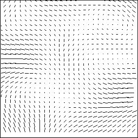
Figure 8 - Example of a filter with elastic distortions with sigma=4.0 and alpha=8.0
Creating a wrapper to create multiple elastic filters at once:
def _create_elastic_filters(n_filters, sigma=4.0, alpha=8.0):
    return [_create_elastic_distortions(sigma, alpha) for _ in xrange(n_filters)]
The default values are the one that best worked on the Research project. The next step is to create a function that will apply an elastic distortion to an image. Regarding image processing, the best way is to preprocess the dataset images before starting training sessions. If we decided to create distorted images during training, we would do the operation hundreds of time based on the number of epochs we chose (300 in this guide). To be more efficient, we will then create all the distorted images before training and even before constructing the network. Consequently, the images we will manipulate are 28x28 pixels. Here is an implementation of the algorithm to apply distortions to an image:
# Applies an elastic distortions filter to image
def _apply_elastic_distortions(image, filter):
    # Ensures images are of matrix representation shape
    image = np.reshape(image, (28, 28))
    res = np.zeros((28, 28))

    # filter will come out of _create_elastic_filter
    f_x, f_y = filter

    for i in xrange(28):
        for j in xrange(28):
            dx = f_x[i][j]
            dy = f_y[i][j]

            # These two variables help refactor the code
            # They are a little mind tricky; don't hesitate to take a pen and paper to visualize them
            x_offset = 1 if dx >= 0 else -1
            y_offset = 1 if dy >= 0 else -1

            # Retrieving the two closest x and y of the pixels near where the arrow ends
            y1 = j + int(dx) if 0 <= j + int(dx) < 28 else 0
            y2 = j + int(dx) + x_offset if 0 <= j + int(dx) + x_offset < 28 else 0
            x1 = i + int(dy) if 0 <= i + int(dy) < 28 else 0
            x2 = i + int(dy) + y_offset if 0 <= i + int(dy) + y_offset < 28 else 0

            # Horizontal interpolation : for both lines compute horizontal interpolation
            _interp1 = min(max(image[x1][y1] + (x_offset * (dx - int(dx))) * (image[x2][y1] - image[x1][y1]), 0), 1)
            _interp2 = min(max(image[x1][y2] + (y_offset * (dx - int(dx))) * (image[x2][y2] - image[x1][y2]), 0), 1)

            # Vertical interpolation : for both horizontal interpolations compute vertical interpolation
            interpolation = min(max(_interp1 + (dy - int(dy)) * (_interp2 - _interp1), 0), 1)

            res[i][j] = interpolation

    return res
An example of the impact of this function on an image given a filter:

Figure 9 - Example of a elastic distortions transformation on a image from MNIST dataset with sigma=3.0 and alpha=8.0
Since we want to process the dataset images before training, we create a function that will link every function we created for distortions to preprocess the MNIST dataset. We have to be careful to match the labels according to the distorted images: a distorted image has the same label than the original image (it is just distorted in order to mimic the human hand muscles).
# Creates and apply elastic distortions to the input
# images: set of images; labels: associated labels
def expand_dataset(images, labels, n_distortions):
    distortions = _create_elastic_filters(n_distortions)

    new_images_batch = np.array(
        [_apply_elastic_distortions(image, filter) for image in images for filter in distortions])
    new_labels_batch = np.array([label for label in labels for _ in distortions])

    # We don't forget to return the original images and labels (hence concatenate)
    return np.concatenate([np.reshape(images, (-1, 28, 28)), new_images_batch]), \
           np.concatenate([labels, new_labels_batch])
We will need to retrieve batches of (images, labels) for the training sessions. For the raw MNIST dataset, it is implemented as a method of the associated class. Here, for simplicity, we create a batch selector using a new argument that tells the function where to begin picking images and labels (instead of using an iterator, which would probably be the correct way to perform such behaviour):
# Returns a batch from (images, labels) begining at begin ending at begin+batch_size-1 (included)
def get_batch(images, labels, begin, batch_size):
    return images[begin: begin+batch_size], labels[begin: begin+batch_size]
Let’s put all those functions in a file preprocessing.py in the same folder as the main.py file. To incorporate preprocessing into our program, we need to slightly modify the function main. The next piece of code belongs to the function main of the file main.py. I have put in comments the lines that need to be modified and their modifications below (don’t forget to add an empty file init.py in the folder in order to import the file preprocessing.py):
from preprocessing import expand_dataset, get_batch

def main():
    mnist = input_data.read_data_sets('tmp/data', one_hot=True)
    # Add this line: here we decide to use 2 elastic filters (you can change this number if you want)
    images, labels = expand_dataset(mnist.train.images, mnist.train.labels, 2)

    ...
        ...
            ...
            #while current_batch * batch_size <= len(mnist.train.images):
            while current_batch * batch_size <= len(images):
                ...

                #batch_x, batch_y = mnist.train.next_batch(batch_size)
                batch_x, batch_y = get_batch(images, labels, current_batch-2, batch_size)

                ...
The expansion of the dataset is a long process. We only two filters, it takes more than 30 minutes on my computer. With sufficient computation capacity, one could parallelize the expansion in order to reduce its duration down to th where is the desired number of filters (here, it is sequential).
This is it for this post! I hope you learned interesting things :-). If you want to give me feedback about this post, to point some mistakes, to propose improvements or just to speak with me, you can contact me with the icons in the top-right (mail, Github, Linkedin).